Öktem and Romps, Prediction for cloud spacing confirmed using stereo cameras, JAS, 2021
Errata
In equation (9), κ should be k. In the last line of page 3723, the second CW/LCL should be CS/LCL. Both of these have been fixed in the PDF below.
Paper
Description
What sets the sizes of clouds and the spacing between them? For shallow cumulus, we can at least offer an order-of-magnitude answer to this question: the natural length scale in a field of shallow cumulus is the depth of the boundary layer. For shallow (i.e., thin) cumulus, the depth of the boundary layer is approximately equal to the height above ground of the lifting condensation level (LCL). The LCL, in turn, is primarily a function of the near-surface relative humidity. For example, a typical summertime near-surface relative humidity of 60% puts the LCL at a height of about 1 km, so we should expect that shallow-cumulus widths and spacings will be around that length scale.
Unfortunately, this hand waving is a bit uncomfortable. If we think a bit more deeply about the problem, we realize there is at least one other length scale in the problem that we have ignored: the turbulent diffusivity κ (units of m/s2) divided by the square of the Brunt-Väisälä frequency |N2| (units of 1/s2). Why do the clouds not set their sizes and spacing equal to κ|N2|? For that matter, what is the value of κ|N2|?
Thuburn and Efstathiou (2020) offered an answer to this question with a derivation that incorporates the boundary-layer depth, κ, and N2. The idea behind their derivation is that heating of a boundary layer from below (i.e., heating of the ground by the sun) will tend to make the boundary layer unstable to convection (i.e., negative N2). But the more vigorously the boundary layer convects, the higher the turbulent diffusivity κ, and a κ that is high enough will damp the convection to zero. Using the empirical fact that convection tends to very nearly eliminate the convective instability, we may approximate κ as the value that is just big enough to make the most unstable mode of convection have a growth rate of zero (this is called the marginal-stability hypothesis). This leads to a soluble set of equations that predicts that the wavelength of the most unstable mode, which should manifest as the spacing between clouds, is 2√2 times the LCL height.
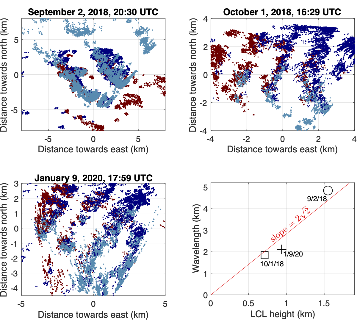
In this paper, we use stereo photogrammetry to test this prediction, and it turns out to work surprisingly well. We generated stereo reconstructions of shallow-cumulus events from 129 days at the DOE site in Oklahoma. Compositing those events, we find that, compared to 2√2 ≅ 2.8, the ratio of the cloud spacing to the LCL height tends to hover around 2.7 to 3.1. If we focus exclusively on cloud streets, which are closer analogs to the two-dimensional calculation that leads to 2√2, we again find very good agreement.
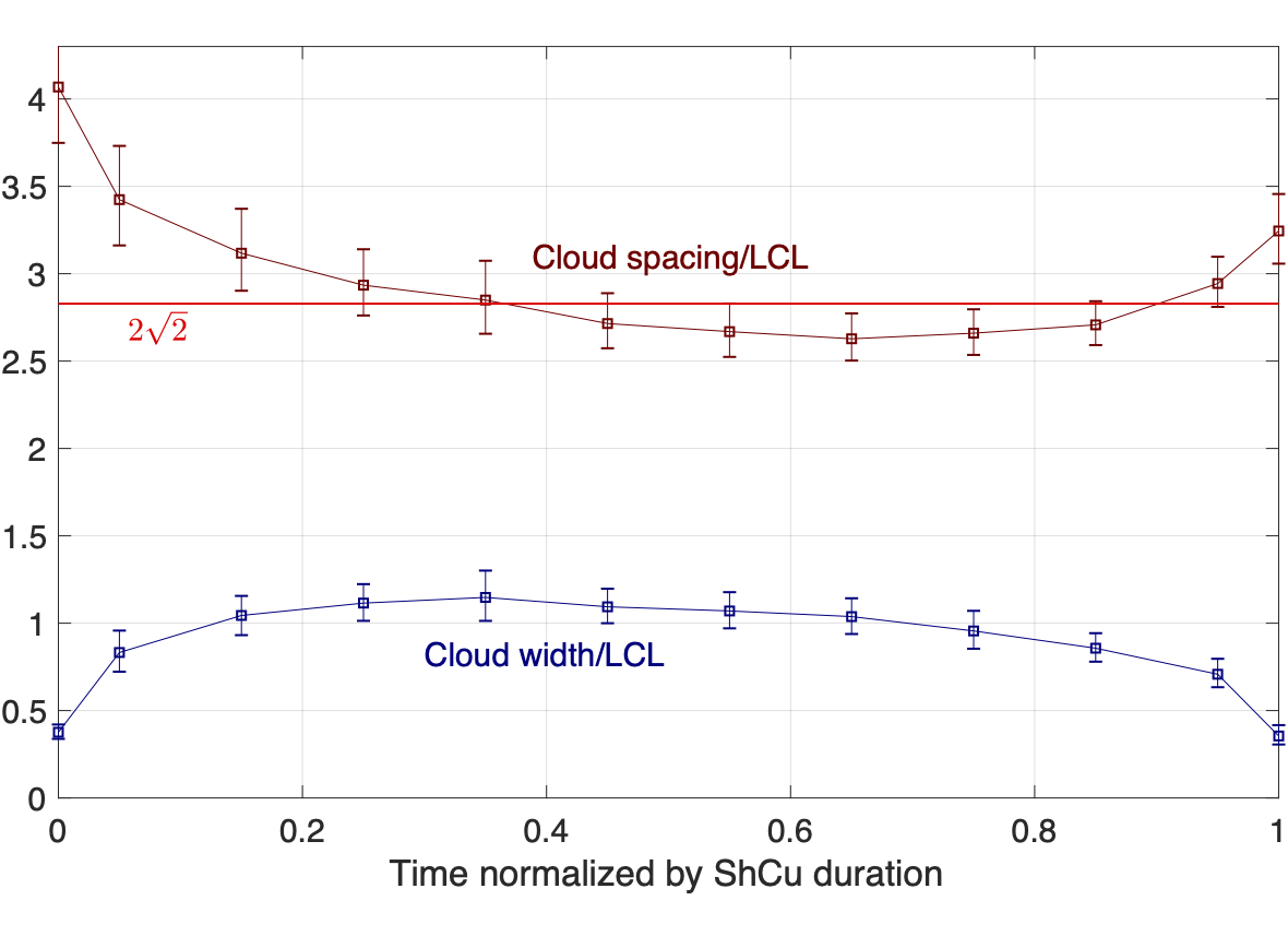
Composite evolution of cloud spacing and cloud width from the onset (t=0) to the termination (t=1) of shallow cumulus as observed by the stereo cameras during 129 such events. The red solid line shows the prediction of Thuburn and Efstathiou (2020).
(top and left) Horizontally projected cloud streets from the raw stereo-camera data at three moments in time. Data from the northwest, northeast, and southern camera pairs are shown as red, dark-blue, and light-blue dots, respectively. (lower right) The best-fit horizontal wavelengths plotted against the LCL height. The straight line shows the predicted slope of 2√2.